
 Hybrid architectures are popular. As I look across the organizations that I consult with, I am hard pressed to point out many that aren’t working in some flavor of hybrid environment, even if they don’t realize it. One of the things that can become confusing is the overall availability of a solution when parts of it reside on-premise and parts of it reside in a public cloud. Fully understanding the implications as it relates to your overall availability is going to affect how you architect these systems. We are going to get our arms around availability here, and maybe do some math to help quantify it.
First, lets start by getting an understanding of the availability of our individual services, then we will build upon it. Take your mean time between failures (MTBF) multiplied by your mean time to repair (MTTR) to figure out your projected availability. Include outages caused by disruptive maintenance. For example, if a server has 2 incidents in a year, and each one caused a 1 hr outage, that represents a 182 day MTBF with a MTTR of 1hr to project an availability of about 99.977%.
Availability is commonly expressed as a percentage, but here is a quick chart to equate it with time:
| Percentage | Downtime Per Year |
| 99% | 3.6 Days |
| 99.9% | 8.77 Hours |
| 99.99% | 52.5 Minutes |
| 99.999% | 5.2 Minutes |
| 99.9999% | 31.5 Seconds |
To figure out other values, you can use the calculator here.
Now, lets talk about systems. In real life, our systems are comprised of multiple services with varying levels of availability. So, while we figured out that the example server above is 99.977% available, it probably doesn’t stand alone. It relies on a network, maybe storage, maybe other servers or services. So, if we want to understand the true availability of the entire system, we have to do some math.
There are 2 main ways we can combine components: in series, and in parallel.
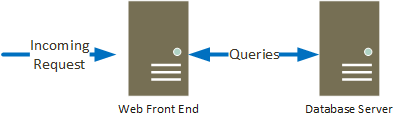
First, components in series. This is when BOTH components need to be available in order for a system to work. These could be considered hard dependencies. If either component goes down, the whole solution is unavailable, such as shown in the image below. The practical impact of this is that the overall availability of the system is lower than the availability of any 1 component. The reason for this is that it is unlikely that failures in the various components will occur at the same time. So, you need to figure out an overall availability for the system that takes both components into account.
Calculating availability for these components is easy:
Ax * Ay * Az … An
So. Lets say that both of these servers have 99.9% uptime. In our example above, that would be:
.999 * .999 = .998.
This tells us that the overall availability for the system shown above with 2 components is 99.8%, which is about 17.5 hrs a year of downtime.
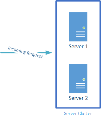
Now, on to parallel systems. These are systems where the service is available even if one of the components fails. Clusters can be examples of parallel systems. The practical impact of this is that the availability for a system made with components in parallel is that the overall availability of the system is higher than that of the individual components. Shown below.
 To calculate availability for systems like this, it looks like:
1 – (1-(Ax * Ay)n)
So, if we stick with 99.9% available components in this example, our equation would be:
1-(1-(.999 * .999)2 = 99.9999%
This tells us that the overall availability for the system above is 6 x 9’s, which is about 31 seconds a year. That is a lot less downtime than the 8.7hrs you get from those components individually at 99.9%!
Ok, now that you know the math, I’ll save you from having to do it. You can work out simple variations on availability problems like this on the calculators page here.
What if you have an application that relies on a component located on-premise, as well as a service located in a public cloud? Lets use AWS EC2 as an example. They publish the availability targets for this service here. AWS offers a 99.99% target for EC2, EBS, and ECS. This would represent a hard dependency, which would fall into the serial category. If we stick with the 99.9% metric from the example above, and combine it with a 99.99% target from the cloud service we are dependent on, it would look like this:
.999 * .9999 = 99.89%
99.89% availability is about 9h 38m of downtime in a year, which is a good bit more downtime than just a 99.9% available service. So, even though we are building on a service with a relatively high level of availability, combining them poses a significant reduction in our projected availability. This excludes other SLAs that may also be in the loop, such as connectivity and related devices.
The takeaway here is that you need to build your environments with parallel systems, even when you are building for the public cloud, to achieve high levels of availability. Looking at the published SLA’s and targets for public cloud services, you can tell that it will require some additional redundancy in the form of parallel components to reach the 5 x 9’s range which has become the goal for many on-premise systems.